Clusters

The goal of this analysis is to dig deeper into the ordinations produced in Preliminary Analysis. In particular, we are interested in what appears to be two different clusters within the fertilized group. Our goals are:

• Characterize the communities in the two groups/Determine important taxa

Preparing the data

We repeat the data prep from Preliminary Analysis:

Getting the data ready

# TODO: Refactor into import_data.R

data.priming <- read.csv(here("data", "priming_amoA_deltaCt.csv"), header = T) %>% 
  rename(sample_id = X) 

data.raw <- read.csv(here("data", "priming_amoA_rawCt.csv"), header = T) %>% 
  rename(sample_id = X)

data.priming.long <- data.priming %>% 
  pivot_longer(cols = starts_with("amoA"), names_to = "amoA", values_to = "deltaCT")

data.raw.long <- data.raw %>% 
  pivot_longer(cols = starts_with("amoA"), names_to = "amoA", values_to = "CT")

data.priming.long$sample_id <- fct_reorder(data.priming.long$sample_id, parse_number(data.priming.long$sample_id))

df <- data.priming[, -1]
rownames(df) <- data.priming[, 1]

metadata <- df %>% 
  select(fert_level:field_rep) %>%
  mutate(across(everything(), as.factor))


amoa_counts <- df %>% 
  select(starts_with("amoA"))

non_detect_counts <- data.raw.long %>%
  group_by(fert_level, amoA) %>% 
  count(CT == 40) %>% 
  rename(non_detect = `CT == 40`) %>%
  filter(non_detect == TRUE)

amoA_organism_info <- readxl::read_xlsx(here("data", "amoa_mfp_qpcr_org_accessions.xlsx"), sheet = 5) %>% 
  select(-c(contains(c("forward", "reverse", "notes")))) 

removes <- non_detect_counts %>% 
  pivot_wider(names_from = fert_level, values_from = n, names_prefix = "fert.") %>%
  filter(fert.0 > 30 & fert.336 > 30) %>%
  pivot_longer(cols = fert.0:fert.336, names_to = "fert_level", values_to = "n")

data.priming.reduced <- data.priming %>% 
   select(-one_of(removes$amoA))

data.priming.reduced.long <- data.priming.reduced %>% 
  select(-sample_id, field_rep) %>% 
  pivot_longer(cols = contains("amoa")) 


amoA_presence_absence <- data.raw %>%
  select(sample_id, starts_with("amoA")) %>% 
  mutate(across(starts_with("amoA"), ~ ifelse(.x == 40, 0, 1))) 

amoa_tax_table <- amoA_organism_info %>% 
  select(array_name, best_blast_hits) %>% 
  column_to_rownames(var = "array_name") %>% 
  tax_table()

estimate_richness_mod <- function(physeq, split=TRUE, measures=NULL){
  

  if( !split ){
    OTU <- taxa_sums(physeq)        
  } else if( split ){
    OTU <- as(otu_table(physeq), "matrix")
    if( taxa_are_rows(physeq) ){ OTU <- t(OTU) }
  }
  

  renamevec = c("Observed", "Chao1", "ACE", "Shannon", "Pielou", "Simpson", "InvSimpson", "SimpsonE", "Fisher")
  names(renamevec) <- c("S.obs", "S.chao1", "S.ACE", "shannon", "pielou", "simpson", "invsimpson", "simpsone", "fisher")

  if( is.null(measures) ){
    measures = as.character(renamevec)
  }

  if( any(measures %in% names(renamevec)) ){
    measures[measures %in% names(renamevec)] <- renamevec[names(renamevec) %in% measures]
  }
  

  if( !any(measures %in% renamevec) ){
    stop("None of the `measures` you provided are supported. Try default `NULL` instead.")
  }
  

  outlist = vector("list")

  estimRmeas = c("Chao1", "Observed", "ACE")
  if( any(estimRmeas %in% measures) ){
    outlist <- c(outlist, list(t(data.frame(estimateR(OTU)))))
  }
  if( "Shannon" %in% measures ){
    outlist <- c(outlist, list(shannon = diversity(OTU, index="shannon")))
  }
  if( "Pielou" %in% measures){
    #print("Starting Pielou")
    outlist <- c(outlist, list(pielou = diversity(OTU, index = "shannon")/log(estimateR(OTU)["S.obs",])))
  }
  if( "Simpson" %in% measures ){
    outlist <- c(outlist, list(simpson = diversity(OTU, index="simpson")))
  }
  if( "InvSimpson" %in% measures ){
    outlist <- c(outlist, list(invsimpson = diversity(OTU, index="invsimpson")))
  }
  if( "SimpsonE" %in% measures ){

    outlist <- c(outlist, list(simpsone = diversity(OTU, index="invsimpson")/estimateR(OTU)["S.obs",]))
  }
  if( "Fisher" %in% measures ){
    fisher = tryCatch(fisher.alpha(OTU, se=TRUE),
                      warning=function(w){
                        warning("phyloseq::estimate_richness: Warning in fisher.alpha(). See `?fisher.fit` or ?`fisher.alpha`. Treat fisher results with caution")
                        suppressWarnings(fisher.alpha(OTU, se=TRUE)[, c("alpha", "se")])
                      }
    )
    if(!is.null(dim(fisher))){
      colnames(fisher)[1:2] <- c("Fisher", "se.fisher")
      outlist <- c(outlist, list(fisher))
    } else {
      outlist <- c(outlist, Fisher=list(fisher))
    }
  }
  out = do.call("cbind", outlist)

  namechange = intersect(colnames(out), names(renamevec))
  colnames(out)[colnames(out) %in% namechange] <- renamevec[namechange]

  colkeep = sapply(paste0("(se\\.){0,}", measures), grep, colnames(out), ignore.case=TRUE)
  out = out[, sort(unique(unlist(colkeep))), drop=FALSE]

  out <- as.data.frame(out)
  return(out)
}

rownames(amoa_tax_table) <- amoA_organism_info$array_name

ps <- phyloseq(
  otu_table(amoA_presence_absence %>% column_to_rownames(var = "sample_id"), taxa_are_rows = FALSE),
  sample_data(metadata),
  amoa_tax_table
)

mds.priming = metaMDS(data.priming.reduced %>% select(contains("amoa")), distance = "bray", k = 3)

site.scores <- as.data.frame(scores(mds.priming, display = "sites")) %>% 
  mutate(sample_id = data.priming.reduced$sample_id,
         Crop = data.priming.reduced$crop,
         Fert_Level = as.factor(data.priming.reduced$fert_level),
         Day = as.factor(data.priming.reduced$doe),
         Substrate_Addition = as.factor(data.priming.reduced$addition))

 

dune_dist <- vegdist(data.priming %>% select(starts_with('amoA')))

amoa_anosim <- anosim(dune_dist, data.priming$fert_level)

mds.spp.fit <- envfit(mds.priming, data.priming.reduced %>% select(contains("amoa")), permutations = 999)

spp.scrs <- as.data.frame(scores(mds.spp.fit, display = "vectors")) 
spp.scrs <- cbind(spp.scrs, Species = rownames(spp.scrs)) 
spp.scrs <- cbind(spp.scrs, pval = mds.spp.fit$vectors$pvals)

spp.scores <- as.data.frame(scores(mds.spp.fit, display = "vectors")) %>% 
  mutate(Species = rownames(.),
         pval = mds.spp.fit$vectors$pvals)

Here is the NMDS in question:

Plotting the NMDS

nmds.plot <- site.scores %>% 
  ggplot(aes(NMDS1, NMDS2, fill = Fert_Level)) +  
  geom_hline(yintercept = 0.0,
             colour = "grey",
             lty = 2) +
  geom_vline(xintercept = 0.0,
             colour = "grey",
             lty = 2) +
  geom_point(size = 4, shape = 21) + 
    theme(
    plot.title = element_text(hjust = 0.5),
    legend.text = element_markdown(size = 12),
    legend.title = element_markdown(size = 12, hjust = 0),
    axis.text.x = element_text(size = 14),
    axis.text.y = element_text(size = 14),
    axis.title.x = element_text(size = 12),
    axis.title.y = element_text(size = 12),
    panel.grid = element_line(color = "gray95"),
    panel.border = element_rect(color = "black", size = 1, fill = NA)
  ) +
  scale_fill_discrete(name = "Fertilizer Level<br>
                              <span style = 'font-size:8pt;'>
                              (kg N ha<sup>-1</sup> y<sup>-1</sup>)
                              </span>") +
  guides(
    fill = guide_legend(override.aes = list(shape = 21, size = 5))
  ) 

nmds.plot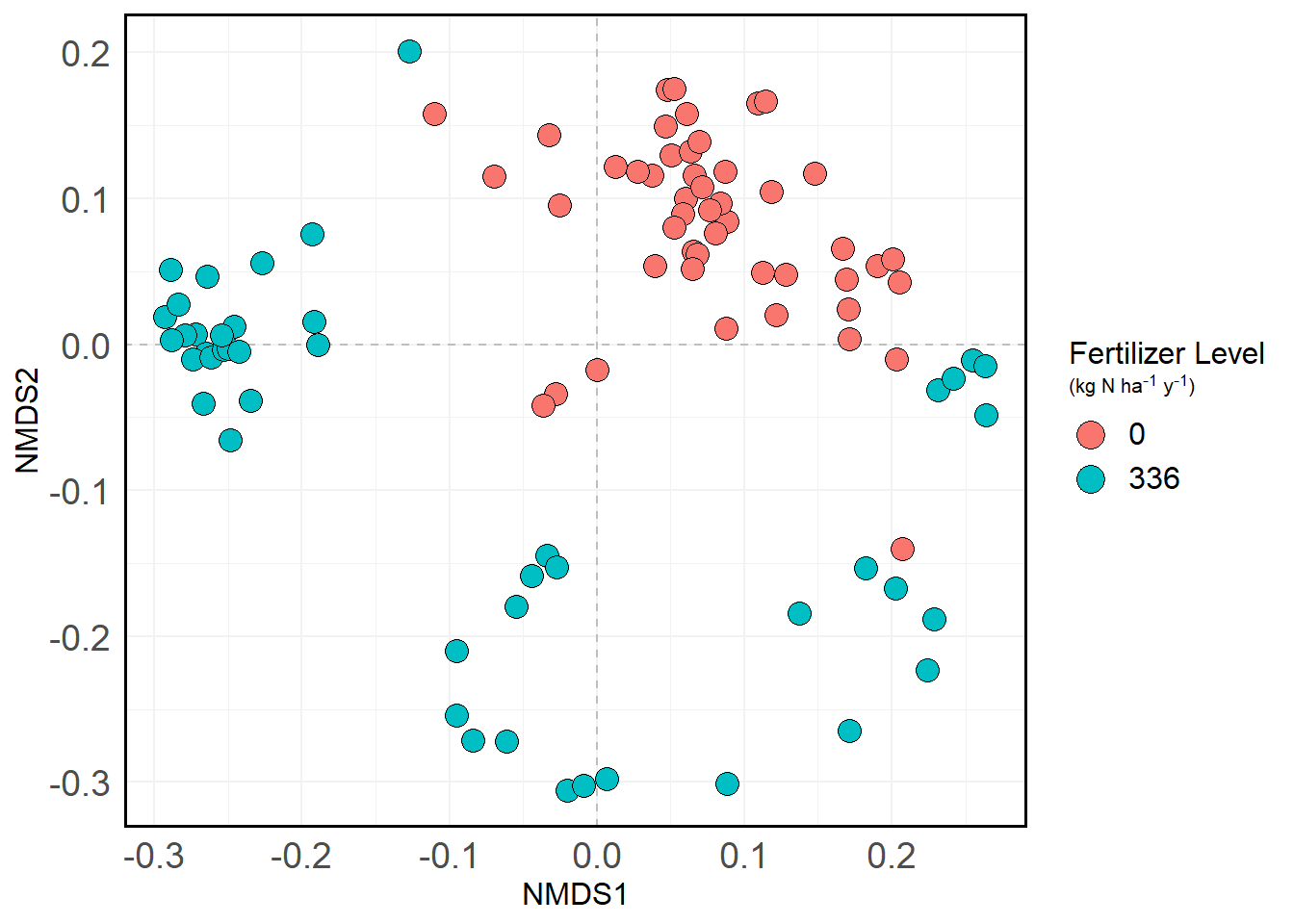

Within the fertilized group, there appears to be three interesting clusters:

• One on the left, which we’ll call Cluster 1
• One in the bottom center, which we’ll call Cluster 2
• And the vague one in the bottom right, which we’ll call Cluster 3

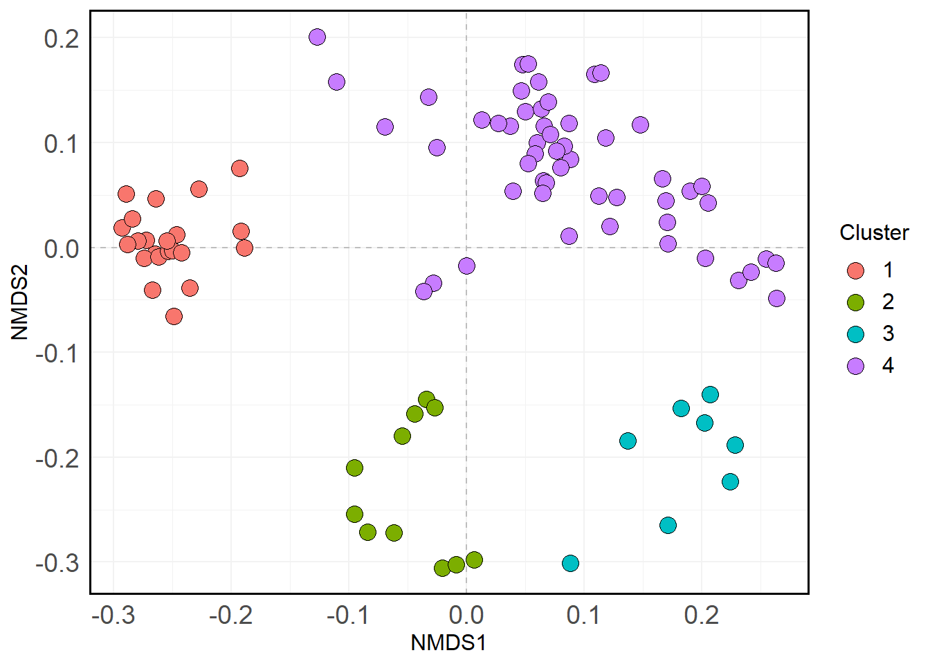
We’ll group everything else into Cluster 4 (the “leftovers”). Here’s what that looks like.

Code

site.scores <- site.scores %>% 
  mutate(Cluster = as.factor(case_when(
    NMDS1 < -0.15 ~ 1,
    NMDS2 < -0.1 & NMDS1 < 0.05 ~ 2,
    NMDS2 < -0.1 & NMDS1 > 0.05 ~ 3,
    TRUE ~ 4
  ))) 

site.scores %>% 
  ggplot(aes(NMDS1, NMDS2, fill = Cluster)) +  
  geom_hline(yintercept = 0.0,
             colour = "grey",
             lty = 2) +
  geom_vline(xintercept = 0.0,
             colour = "grey",
             lty = 2) +
  geom_point(size = 4, shape = 21) + 
    theme(
    plot.title = element_text(hjust = 0.5),
    legend.text = element_markdown(size = 12),
    legend.title = element_markdown(size = 12, hjust = 0),
    axis.text.x = element_text(size = 14),
    axis.text.y = element_text(size = 14),
    axis.title.x = element_text(size = 12),
    axis.title.y = element_text(size = 12),
    panel.grid = element_line(color = "gray95"),
    panel.border = element_rect(color = "black", size = 1, fill = NA)
  ) 

Let’s update the phyloseq object with this cluster info:

sample_data(ps) <- metadata %>% rownames_to_column(var = "sample_id") %>% 
  left_join(site.scores) %>% 
  select(-crop) %>% 
  column_to_rownames("sample_id")

Alpha diversity

We’ll start by looking at differences in alpha diversity between the clusters.

Calculate richness, do pairwise Kruskal-Wallis, and plot

metrics <- c("Observed", "Shannon")
richness <- estimate_richness_mod(ps, measures = metrics) %>% 
  rownames_to_column(var = "sample_id") %>% 
  mutate(sample_id = str_sub(sample_id, start = 2)) 

richness <- left_join(sample_data(ps) %>% data.frame() %>% rownames_to_column(var = "sample_id"), richness) %>% 
  pivot_longer(cols = Observed:Shannon, names_to = "Metric", values_to = "Value")

samples_richness_clusters <- richness %>% 
  pivot_wider(names_from = "Metric", values_from = "Value") %>% 
  select(sample_id, Observed, Shannon, Cluster)

comparisons <- crossing(1:4, 1:4, .name_repair = "minimal") %>% 
  rename(Cluster_1 = 1, Cluster_2 = 2) %>% 
  filter(Cluster_1 != Cluster_2) %>% 
  mutate(group = if_else(Cluster_1 < Cluster_2, paste0(Cluster_1, Cluster_2), paste0(Cluster_2, Cluster_1))) %>% 
  group_by(group) %>% 
  slice_head(n = 1) %>% 
  ungroup() %>% 
  select(-group)

# Doesn't want to be a function for some reason...
# pairwise_kruskal <- function(metric) {
#   apply(comparisons, 1, function(x) broom::tidy(kruskal.test({{ metric }} ~ Cluster, data = samples_richness_clusters %>% filter(Cluster %in% c(x['Cluster_1'], x['Cluster_2']))))) %>% 
#   bind_rows() %>%
#   bind_cols(comparisons) %>% 
#   mutate(metric = {{ metric }})
# }
# 
# pairwise_kruskal("Observed")


observed <- apply(comparisons, 1, function(x) broom::tidy(kruskal.test(Observed ~ Cluster, data = samples_richness_clusters %>% filter(Cluster %in% c(x['Cluster_1'], x['Cluster_2']))) )) %>% 
  bind_rows() %>%
  bind_cols(comparisons) %>% 
  mutate(metric = "Observed")

shannon <- apply(comparisons, 1, function(x) broom::tidy(kruskal.test(Shannon ~ Cluster, data = samples_richness_clusters %>% filter(Cluster %in% c(x['Cluster_1'], x['Cluster_2']))) )) %>% 
  bind_rows() %>%
  bind_cols(comparisons) %>% 
  mutate(metric = "Shannon")


p.values <- bind_rows(observed, shannon) %>% 
    mutate(sig = case_when(
    p.value < 0.05 & p.value > 0.01 ~ "*",
    p.value < 0.01 & p.value > 0.001 ~ "**",
    p.value < 0.001 ~ "***",
    TRUE ~ "NS"
  )) 

summaries <- richness %>% 
  group_by(Metric, Cluster) %>% 
  summarize(mean_val = mean(Value), 
            sd_val = sd(Value),
            n = n(),
            .groups = "drop") %>% 
  mutate(se = abs((sd_val / sqrt(n)) * qt(0.025, n - 1) )) %>% 
  mutate(ymax = mean_val + se, 
         ymin = mean_val - se) %>% 
  bind_cols(
    "labels" = rep(c("a", "b", "c", "d"), 2)
  ) %>% 
  mutate(offset = ifelse(Metric == "Observed", 2.2, 0.20))

summaries %>%  
  ggplot(aes(Cluster, mean_val, fill = Cluster)) + 
  geom_col(color = "black", size = 1) +
  facet_wrap(~ Metric, scales = "free_y") + 
  theme(
    legend.position = "none",
    strip.background = element_blank(),
    axis.title.y = element_blank(),
    strip.placement = "outside",
    plot.title = element_text(hjust = 0.5),
    strip.text.y = element_text(face = "bold", size = 10),
    strip.text = element_text(face = "bold", size = 10),
    panel.grid.major.x = element_blank(),
    panel.grid.minor.x = element_blank(),
    panel.grid.minor.y = element_blank(),
    panel.grid.major.y = element_line(color = "gray90", linetype = "dashed"),
    axis.ticks = element_blank(),
    panel.border = element_rect(color = "black", size = 1, fill = "NA")
  ) +
  scale_y_continuous(expand = expansion(mult = c(0, 0.1))) + 
  geom_errorbar(aes(ymin = ymin, ymax = ymax, width = 0.5)) + 
  geom_text(
    aes(y = ymax + offset, label = labels),
    size = 5
    ) +
  labs(
    x = "Gene cluster",
    title = "Alpha diversity metrics by Cluster"
  )

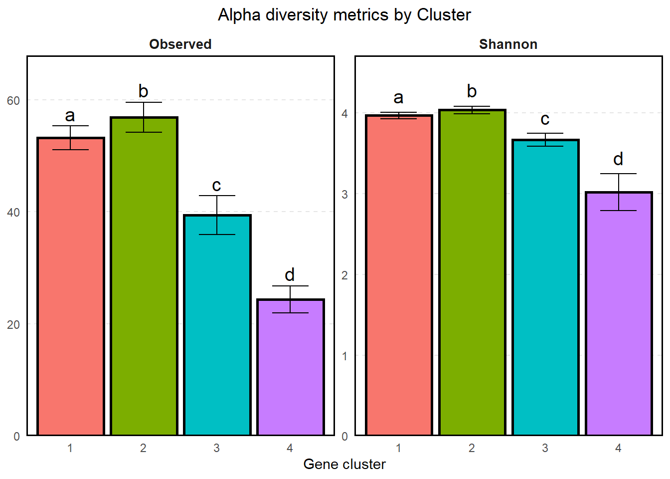
So according to our pairwise Kruskal-Wallis, each of the clusters has significantly different observed diversity and shannon diversity. In particular, Cluster 4 (the “leftover” cluster) has significantly lower observed/shannon diversity than Cluster 3 (the “vague” cluster), which has lower diversity than the other two clusters. While I’m inclined to believe that that alpha diversities of 4 is less than the alpha diversities of 3, which is in turn lower than the other two, the 95% CIs overlap for Clusters 1 and 2 and I wouldn’t conclude anything there.

Which genes are different between clusters?

If we were just comparing the abundances between two clusters or groups, I could do a differential barchart like the ones at the bottom of this section. Unfortunately, since we have four groups, that doesn’t quite make sense. For now, we’ll just visualize with a heatmap.

all_data_long <- ps %>% 
  sample_data() %>% 
  data.frame() %>% 
  rownames_to_column(var = "sample_id") %>% 
  left_join(
    ps %>% 
      otu_table() %>% 
      data.frame() %>% 
      rownames_to_column(var = "sample_id")
  ) %>% 
  pivot_longer(cols = starts_with("amoA"), names_to = "amoA", values_to = "presence")

all_data_long %>% 
  group_by(amoA, Cluster) %>% 
  summarize(mean_presence = mean(presence)) %>% 
  mutate(amoA = str_sub(amoA, -2)) %>%
  ggplot(aes(Cluster, amoA, fill = mean_presence)) + 
  geom_tile(color = "black", aes()) + 
  coord_fixed(ratio = 0.4) + 
  scale_fill_viridis_c(option = "cividis") + 
  labs(
    fill = "Mean Presence"
  )

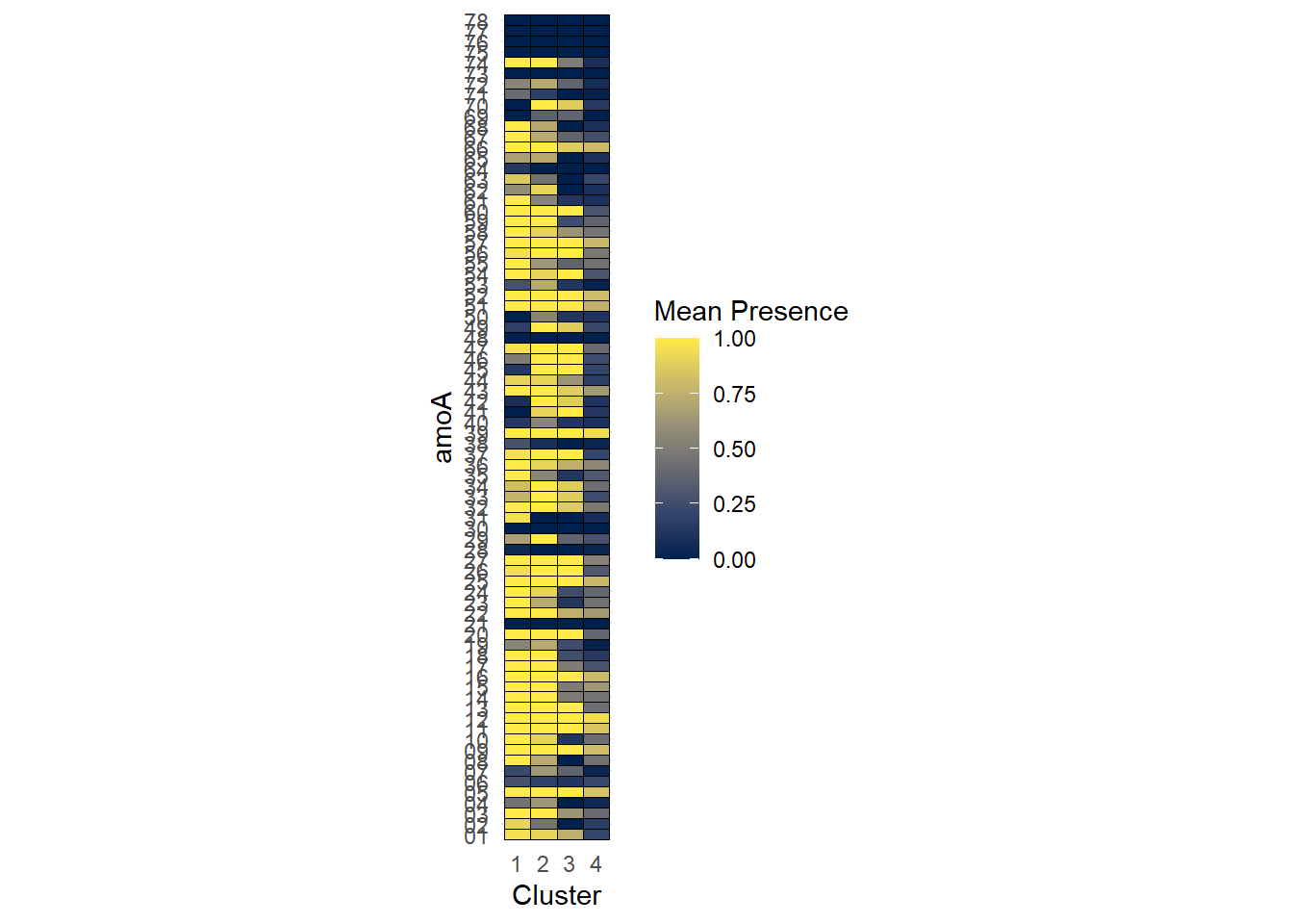
This reinforces our pairwise tests for differences in alpha diversity above - cells in the Cluster 4 column are typically darker than the other columns, indicating that there are fewer genes present there.