Differential Abundance Analysis of Bacteria
library(phyloseq, warn.conflicts = FALSE)
library(data.table, warn.conflicts = FALSE)
library(RColorBrewer, warn.conflicts = FALSE)
library(ggplot2, warn.conflicts = FALSE)
library(igraph, warn.conflicts = FALSE)
library(vegan, warn.conflicts = FALSE)
library(vegetarian, warn.conflicts = FALSE)
I have a filter to remove samples with total abundances of less than 200.. this isn’t necessary with this data, since it has been rarefied to 500, btu is good practice none-the-less. Also I remove taxa that have abundance less than 2 across all samples. Again, the choice to do this is dependent on your interests in the data.
phylo.data <- readRDS("data/rare_b.rds")
phylo.data <- prune_samples(sample_sums(phylo.data)>=200, phylo.data)
phylo.data <- filter_taxa(phylo.data, function(x) sum(x) >= 2, T)
metadata <- sample_data(phylo.data)
Alpha Diversity
Calculated using Shannon index \(H = \sum_{i=1}^{R}\ln{p_{i}}\), it is seen that the treatments allowing more dispersal show greater diversity (increased diverstiy being values less than \(1\)).
richness <- plot_richness(phylo.data, measures = "Shannon")$data
p <- ggplot(richness, aes(x = Treatment, y = value), color = Treatment)
  p <- p + geom_boxplot(aes(color = Treatment), position = "dodge")
  p <- p + ggtitle("Alpha-Diversity of Treatments")
  p <- p + ylab("Shannon Alpha-Diversity")
  p <- p + theme(plot.title = element_text(hjust = 0.5),
                 axis.title.x = element_blank(),
                 legend.position="none")
p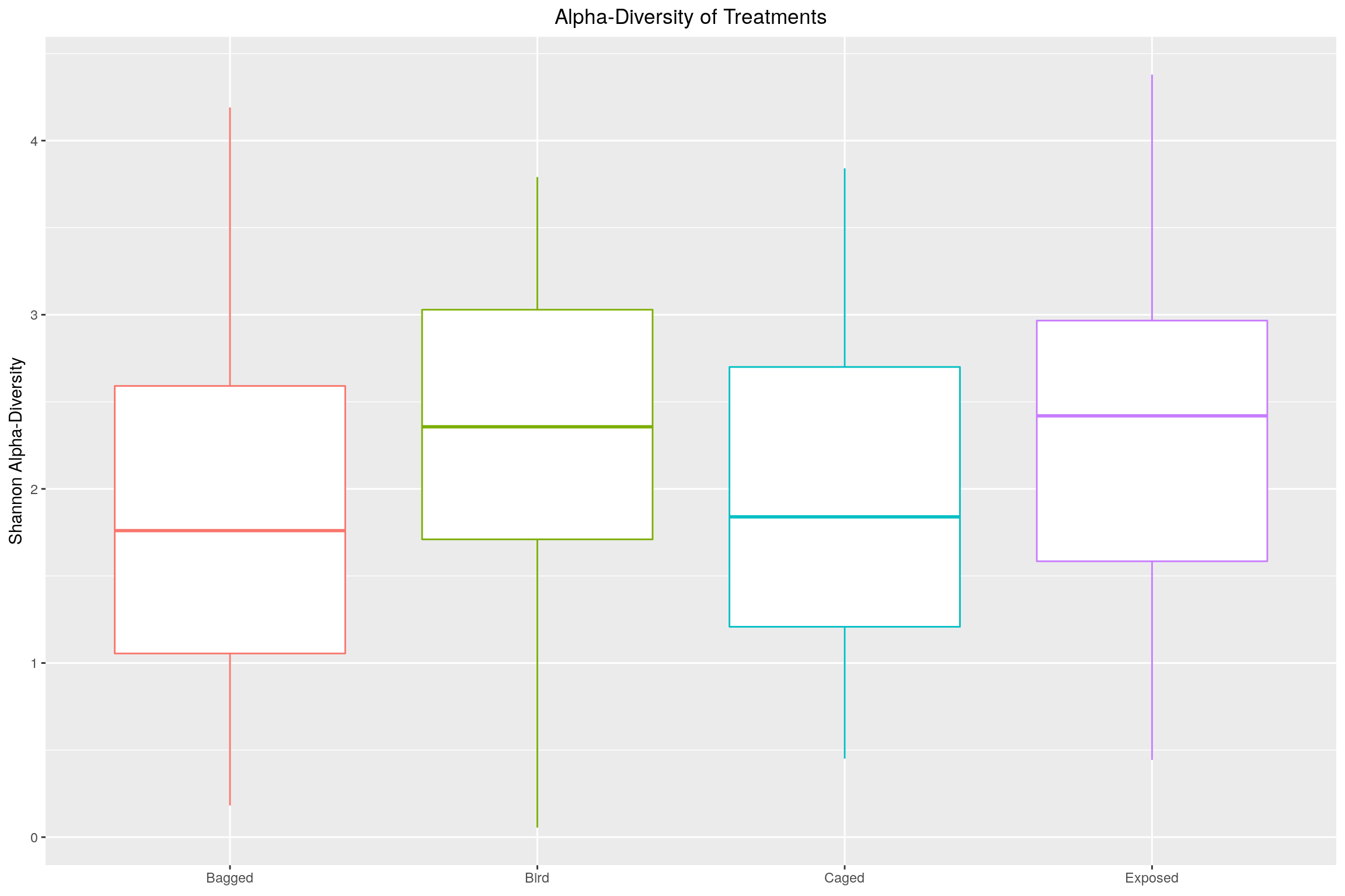
Normalization
The data has already been rarefied to 500, so normalization is not necessary, but normally would be with raw data.
Ordination
MDS plots show us the variation between samples and when looked at by treaments, shows us how much variation exists between each. The circles attempt to show a cluster for the center of the treatment, and we can see how they differentiate, though not to a great extent.
source("scripts/ggplot.NMDS.ellipse.R")
abundances <- otu_table(phylo.data)
getPalette = colorRampPalette(brewer.pal(8, "Dark2")); colorCount = length(unique(metadata$Treatment)); colors = getPalette(colorCount); theme_set(theme_bw())
totu<-t(abundances)
mds <- metaMDS(totu, autotransform = F, k = 2, trymax = 100)
ggplot.NMDS.ellipse(mds, metadata$Treatment, colors)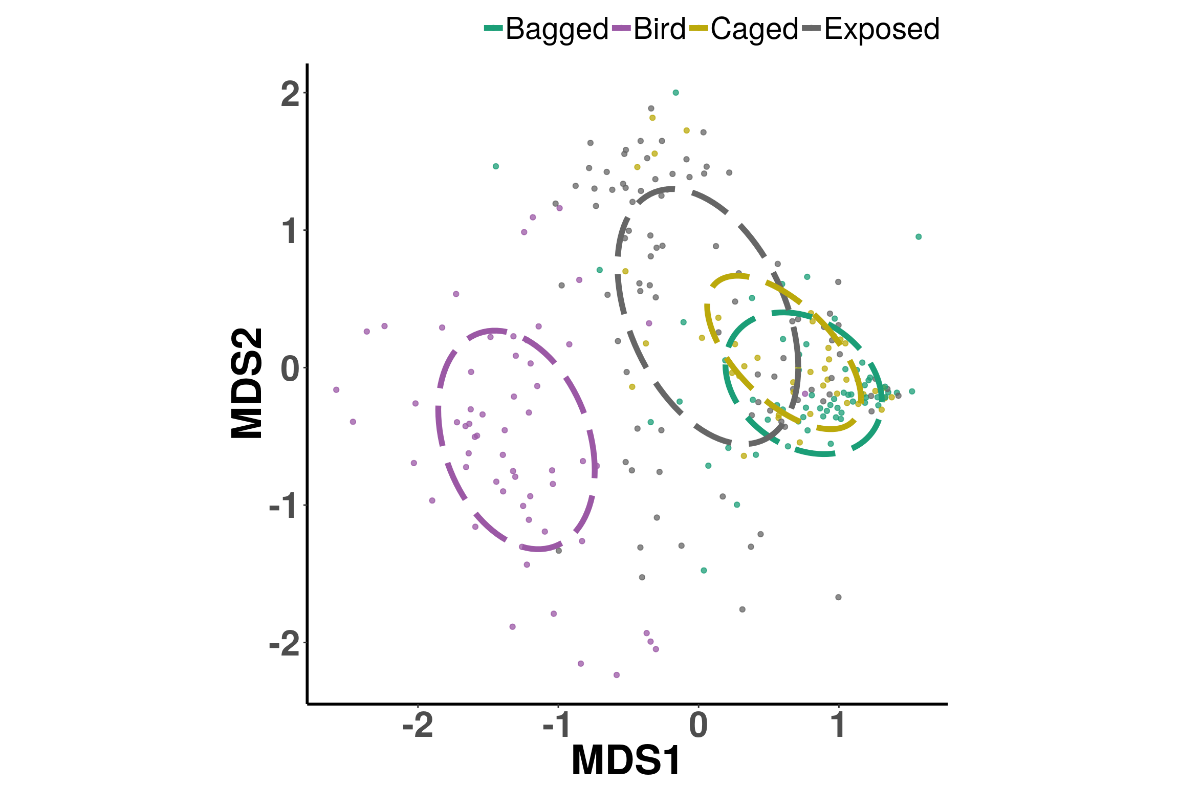
Analysis of variance
Adonis is a method commonly used for ecological systems. It runs permutations of subsets of the data and calculates distances from the cnetroid using in the same manner as ANOVA. And thusly, we find that none of the treatments actually show statistically significant effects on the bacterial community.
rela.dist <- phyloseq::distance(phylo.data, "bray")
si <- data.frame(metadata)
pairs <- t(combn(unique(si$Treatment), 2))
df <- data.frame()
for (i in 1:nrow(pairs)){
    temp.rowname <- paste(pairs[i, 1], pairs[i, 2], sep="::")
    temp.phy <- subset_samples(phylo.data, Treatment %in% pairs[i, ])
    temp.phy <- prune_taxa(taxa_sums(temp.phy) > 0, temp.phy)
    temp.dist <- phyloseq::distance(temp.phy, "bray")
    temp.result <- adonis(temp.dist ~ Treatment, perm=9999, as(sample_data(temp.phy), "data.frame"))
    temp.df <- data.frame(temp.rowname, temp.result$aov.tab[4][1, ], temp.result$aov.tab[5][1, ], temp.result$aov.tab[6][1, ])
    df <- rbind(df, temp.df)
}
names(df)<-c("factor", "rela.F.model", "rela.adonis_R2", "rela.Pr(>F)")
df
## factor rela.F.model rela.adonis_R2 rela.Pr(>F)
## 1 Bird::Bagged 34.360148 0.22404874 0.0001
## 2 Bird::Exposed 17.684383 0.10609502 0.0001
## 3 Bird::Caged 25.295436 0.20028781 0.0001
## 4 Bagged::Exposed 15.622980 0.09432857 0.0001
## 5 Bagged::Caged 1.465155 0.01416085 0.1468
## 6 Exposed::Caged 8.133569 0.05804154 0.0001Beta-Diversity
Using the \(\beta\)-diversity function published in Vannette et al, We caclulated the \(\beta\)-diversity for each treatment to try to replicate their results.
source("scripts/mds.envfit.arrows.R");source("scripts/ordi.sf.R");source("scripts/Vannette.R");source("scripts/Tello.R");
caged <- subset_samples(phylo.data, Treatment=="Caged")
caged <- prune_taxa(taxa_sums(caged) > 0, caged)
bagged <- subset_samples(phylo.data, Treatment=="Bagged")
bagged <- prune_taxa(taxa_sums(bagged) > 0, bagged)
exposed <- subset_samples(phylo.data, Treatment=="Exposed")
exposed <- prune_taxa(taxa_sums(exposed) > 0, exposed)
bses_bagged <- beta.ses.list(bagged)
names(bses_bagged) <- rownames(sample_data(bagged))
bses_caged <- beta.ses.list(caged)
names(bses_caged) <- rownames(sample_data(caged))
bses_exposed <- beta.ses.list(exposed)
names(bses_exposed) <- rownames(sample_data(exposed))
betas <- list(bses_bagged,bses_caged,bses_exposed)
names(betas) <- c("bagged","caged","exposed")
saveRDS(betas, "data/bacteria/beta_diversities.RDS")betas <- readRDS("data/bacteria/beta_diversities.RDS")
bses_bagged <- betas$bagged
bses_caged <- betas$caged
bses_exposed <- betas$exposedgetPalette = colorRampPalette(brewer.pal(8, "Dark2"))
colorCount = length(unique(sample_data(phylo.data)$Treatment))
colors = getPalette(colorCount)
datta <- melt(c(data.frame(Bagged = bses_bagged), data.frame(Caged = bses_caged), data.frame(Exposed = bses_exposed))); colnames(datta) <- c('Beta', 'Treatment')
p <- ggplot(datta, aes(x = Treatment, y = Beta), color = Treatment)
p <- p + geom_boxplot(aes(color = Treatment), position = "dodge")
p <- p + ggtitle("Beta-Diversity of Treatments")
p <- p + ylab("")
p <- p + theme(plot.title = element_text(hjust = 0.5),
axis.title.x = element_blank(),
legend.position="none")
p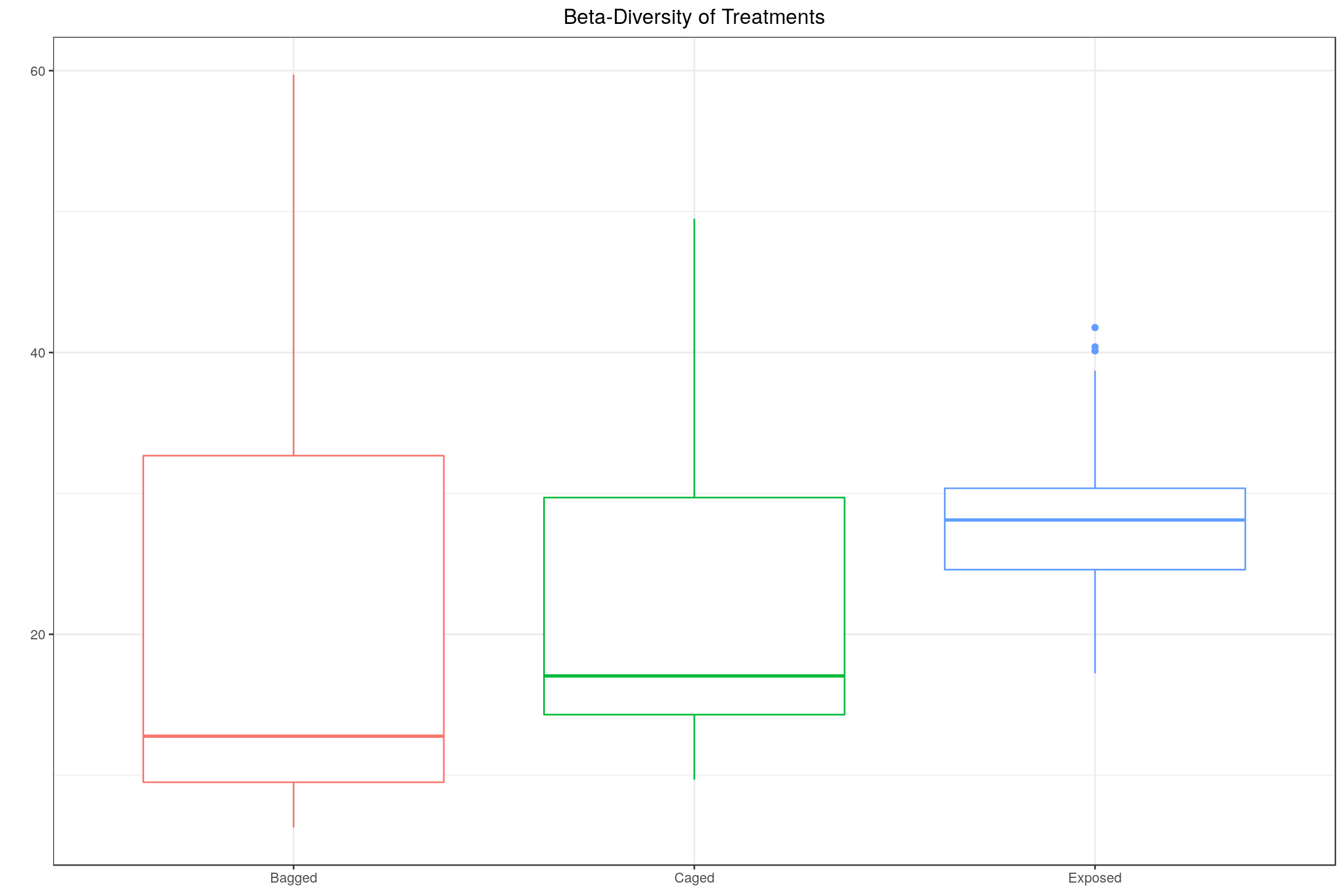
Paul Villanueva and
Schuyler Smith
Ph.D. Students - Bioinformatics and Computational Biology
Iowa State University. Ames, IA.