File manipulation from the command line

I’m currently developing a primer design pipeline for the GERMS lab. The pipeline takes as input a fasta file containing the genes of interest and a directory of metagenomes. The pipeline then clusters the genes, identifies which genes are abundant in the submitted metagenomes, and designs primers for those sequences. See below for an overview of the process:

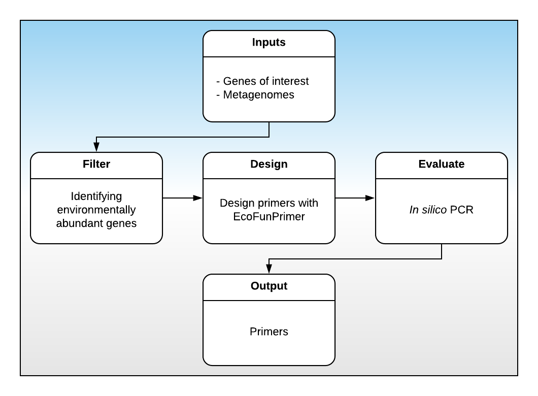
MetaFunPrimer flowchart

Today, we will working on the Filter step. This step is comprised of the following:

1. Choose an optimum similarity threshold for gene clustering
2. Quantify environmental abundance and presence by BLAST the representative sequences against the metagenomes
3. Determine which clusters to include
4. Extract the nucleotide sequences

Querying the sequences against all the metagenomes takes more computational resources and time than are available to us today, so we will only be reproducing steps 1, 3, and 4.

Choosing an optimum similarity threshold for gene clustering

The first step in the filtering process is to choose an optimum clustering threshold for our sequences. Sequences don’t have to be 100% similar to code for the same function, so by clustering the genes together at a lower similarity threshold may allow us to hit all of our gene targets with fewer probes.

To perform the clustering, we have used the CD-Hit program. CD-Hit accepts as input a fasta file and a similarity threshold and sorts the sequences into clusters. The output from this program are in data/cluster_information folder. They are of form x.xx.fa and x.xx.fa.clstr, where:

• x.xx is the similarity threshold
• .fa.clstr contains the clustering information
• .fa contains the sequence of each cluster representative

Now that we have all the clustering information from CD-Hit for our target sequences of varying thresholds, our job is to collect all of this information, use it to select an optimal similarity threshold, and collect the representative sequences for querying against our metagenomes.

Let’s begin with a review of grep.

grep

The grep function searches through a file for a search term. It has the following basic syntax

grep <flags> search_term file

For example, if we wanted to find if the word “summer” was in summer_days.txt, we would do the following:

grep "summer" data/practice_data/summer_days.txt

## Summer days (like the summer days)
## Summer days (like the summer days)
## Summer days (like the summer days)
## Summer days (like the summer days)

This shows us the four lines that the word “summer” was found on. Let’s see what happens when we look for a word that isn’t there:

grep "winter" data/practice_data/summer_days.txt

Nothing pops up, as expected.

grep has a ton of flags that we can pass at the command line, only a few of which we’ll cover today. For example, we can pass the -v flag to invert the match, returning every line on which the match wasn’t found. So, to find all the lines on which “summer” doesn’t appear, we would do:

grep -v "summer" data/practice_data/summer_days.txt

## Summer Days - Sebastian Yatra
## I don't wanna let you go
## I don't wanna let you go
## Why you wanna break my heart?
## Try to be honest
## We can make it on our own
## We can make it on our own
## You just gotta give me time
## Just stay here through August
## 
## Please, believe in me
## Like your wildest dreams
## Like your wildest dreams
## Forever free
## Sail away with me
## Don't leave
## 
## Dance on the ocean
## They be playing our song
## Hold on to meet one more time
## Dance on the ocean
## Don't kiss me goodbye
## Don't know what you think you will find
## 
## Summer days
## Summer days
## 
## Yatra, yatra
## Fue culpa del destino y te quedaste sola
## Te puso en mi camino y nos liego la hora
## Contigo a media noche quiero estar a solas
## Lo que tu quieras te haré
## Mi corazón se estalla tocandote en la playa
## Sintiendo que la arena se convierta en amor
## Y un beso es tan profundo
## Que para los segundos
## Sintiendo que el verano se convierta en amor
## 
## Dance on the ocean
## They be playing our song
## Hold on to meet one more time
## Dance on the ocean
## Don't kiss me goodbye
## Don't know what you think you will find
## 
## Summer days
## Summer days
## 
## Dance on the ocean
## They be playing our song
## Hold on to meet one more time
## Dance on the ocean
## Don't kiss me goodbye
## Don't know what you think you will find
## 
## 
## Summer days

Exercise 1.1

• With our last command, we searched for the all the lines in which the term “summer” doesn’t appear - does the output look correct? Search the man page (via man grep) and look for the flag to make the grep search case-insensitive.
• Use the | operator to pipe the output from the above search to wc. How many lines was summer found on? Is there a smarter way to do this? Hint: check the man page.
• Find the flag to output the line number with the matches.

By default, grep only outputs the lines on which the match was found. This can lead to situations where using the -c flag to count occurrences of a term is inaccurate. For example, let’s find all the lines on which the word “sunday” appears in sunday.txt:

grep -i sunday data/practice_data/sunday.txt

## Sunday (feat. Heize, Jay Park) - GroovyRoom 
## Sunday, Sunday
## Sunday, Sunday
## Sunday, Sunday
## Sunday, the day I look forward to the most
## Sunday, Sunday
## Sunday, Sunday
## Sunday, Sunday
## My Monday to Sunday
## Sunday, Sunday
## Sunday, Sunday
## Sunday, Sunday

Now, let’s see what -c says:

grep -ic sunday data/practice_data/sunday.txt

## 12

We can correct this by using the -o flag, which tells grep to output each occurrence of the search term on a separate line:

grep -io sunday data/practice_data/sunday.txt

## Sunday
## Sunday
## Sunday
## Sunday
## Sunday
## Sunday
## Sunday
## Sunday
## Sunday
## Sunday
## Sunday
## Sunday
## Sunday
## Sunday
## Sunday
## Sunday
## Sunday
## Sunday
## Sunday
## Sunday
## Sunday

From here, we can pipe to wc to get the number of occurrences:

grep -io sunday data/practice_data/sunday.txt | wc -l

##       21

Exercise 1.2

• How many lines does the word “Monday” appear on in monday.txt? How many occurrences of “Monday” are there?

Working with fasta files

Now that we have a bit of practice with grep, let’s return to the problem at hand. The data/sequence_info directory has the nucleotide and protein sequences for our genes of interest. Let’s take a look at them:

head data/sequence_info/amoa_prot.fa

## >BAA92239  coded_by=987..1817,organism=Nitrosomonas sp. TK794,definition=ammonia monooxygenase a
## msifrteeilkaakmppeavhmsrlidavyfpilvvllvgtyhmhfmllagdwdfwmdwkdrqwwpvvtpivgitycsaimyylwvnyrqpfgatlcvvclligewltrywgfywwshyplnfvtpgimlpgalmldftlyltrnwlvtalvgggffglmfxpgnwpifgpthlpivvegtllsmadymghlyvrtgtpeyvrhieqgslrtfgghttviaaffaafvsmlmfavwwylgkvyctaffyvkgkrgrivqrndvtafgeegfpegik
## >BAB84331  coded_by=1073..1861,organism=Nitrosomonas sp. ENI-11,definition=ammonia monooxygenase subunit A2
## mppeavhmsrlidavyfpilivllvgtyhmhfmllagdwdfwmdwkdrqwwpvvtpivgitycsaimyylwvnyrqpfgatlcvvclligewltrywgfywwshypinfvtpgimlpgalmldftmyltrnwlvtalvgggffgvlfypgnwpifgpthlpivvegtllsmadymghmyvrtgtpeyvrhieqgslrtfgghttviaaffsafvsmlmftvwwylgkvyctaffyvkgkrgrivhrndvtafgeegfpegik
## >BAB84328  coded_by=1073..1861,organism=Nitrosomonas sp. ENI-11,definition=ammonia monooxygenase subunit A-1
## mppeavhmsrlidavyfpilivllvgtyhmhfmllagdwdfwmdwkdrqwwpvvtpivgitycsaimyylwvnyrqpfgatlcvvclligewltrywgfywwshypinfvtpgimlpgalmldftmyltrnwlvtalvgggffgvlfypgnwpifgpthlpivvegtllsmadymghmyvrtgtpeyvrhieqgslrtfgghttviaaffsafvsmlmftvwwylgkvyctaffyvkgkrgrivhrndvtafgeegfpegik
## >SET51056  coded_by=1286..2116,organism=Nitrosomonas europaea,definition=ammonia monooxygenase subunit A
## msifrteeilkaakmppeavhmsrlidavyfpiliillvgtyhmhfmllagdwdfwmdwkdrqwwpvvtpivgitycsaimyylwvnyrqpfgatlcvvclligewltrywgfywwshypinfvtpgimlpgalmldftlyltrnwlvtalvgggffgllfypgnwpifgpthlpivvegtllsmadymghlyvrtgtpeyvrhieqgslrtfgghttviaaffsafvsmlmftvwwylgkvyctaffyvkgkrgrivhrndvtafgeegfpegik
## >SDW98167  coded_by=1286..2116,organism=Nitrosomonas europaea,definition=ammonia monooxygenase subunit A
## msifrteeilkaakmppeavhmsrlidavyfpiliillvgtyhmhfmllagdwdfwmdwkdrqwwpvvtpivgitycsaimyylwvnyrqpfgatlcvvclligewltrywgfywwshypinfvtpgimlpgalmldftlyltrnwlvtalvgggffgllfypgnwpifgpthlpivvegtllsmadymghlyvrtgtpeyvrhieqgslrtfgghttviaaffsafvsmlmftvwwylgkvyctaffyvkgkrgrivhrndvtafgeegfpegik

head data/sequence_info/amoa_nuc.fa

## >AB031869  location=987..1817,organism=Nitrosomonas sp. TK794,definition=ammonia monooxygenase a
## gtgagtatatttagaacagaagagatcctgaaagcggccaagatgccgccggaagcggtccatatgtcacgcctgattgatgcggtttattttccgattctggttgttctgttggtaggtacctaccatatgcacttcatgttgttggcaggtgactgggatttctggatggactggaaagatcgtcaatggtggcctgtagtaacacctattgtaggcattacctattgctcggcaattatgtattacctgtgggtcaactaccgtcaaccatttggtgcgactctgtgcgtagtgtgtttgctgataggtgagtggctgacacgttactggggtttctactggtggtcacactatccactcaattttgtaaccccaggtatcatgctcccgggtgcattgatgttggatttcacgctgtatctgacacgtaactggttggtgactgcattggttgggggtggattctttggcctgatgtttnnnccaggtaactggccaatctttggcccgacccatctgccaatcgttgtagaaggaacactgttgtcgatggctgactacatgggtcacctgtatgttcgtacgggtacacctgagtatgttcgtcatattgaacaaggttcattacgtacctttggtggtcacaccacagttattgcggcattcttcgctgcgtttgtatccatgctgatgtttgcagtctggtggtatcttggaaaagtttactgcacagccttcttctacgttaaaggtaaaagaggacgtattgtacagcgcaatgatgttacggcatttggtgaagaagggtttccagaggggatcaaa
## >AB079055  location=1073..1861,organism=Nitrosomonas sp. ENI-11,definition=ammonia monooxygenase subunit A2
## atgccaccggaagcggttcatatgtcacgtctgattgacgcggtttattttccaattctgattgttttgctggtaggtacctaccatatgcacttcatgctgctggcaggtgactgggatttctggatggactggaaagatcgtcaatggtggccggttgtgacaccgatcgtaggaattacctactgctcggcaatcatgtattacctgtgggtcaactaccgccaaccgtttggtgcaacactgtgtgtagtgtgtctgttgattggtgaatggctgacacgttactggggattctactggtggtcacactatcctatcaatttcgtaacaccgggtattatgcttccaggtgcgctgatgctggatttcacaatgtatctgacacgcaactggctggtgacggctctggttgggggtggattcttcggtgtgctgttctatccgggtaactggccgatctttggtccgacacatctgccaatcgtcgtagaaggaacactgttgtcgatggctgactacatgggccatatgtatgttcgtacgggtacacctgagtatgttcgtcatattgagcaaggttcactgcgtacctttggtggacataccacagttattgcagcgttcttctctgcattcgtatcaatgttgatgttcacagtatggtggtatcttggaaaagtttactgtacagcctttttctacgttaaaggtaaaagaggtcgtatcgtacatcgcaatgatgttaccgcattcggtgaagaaggctttccagaggggatcaaa
## >AB079054  location=1073..1861,organism=Nitrosomonas sp. ENI-11,definition=ammonia monooxygenase subunit A-1
## atgccaccggaagcggttcatatgtcacgtctgattgacgcggtttattttccaattctgattgttttgctggtaggtacctaccatatgcacttcatgctgctggcaggtgactgggatttctggatggactggaaagatcgtcaatggtggccggttgtgacaccgatcgtaggaattacctactgctcggcaatcatgtattacctgtgggtcaactaccgccaaccgtttggtgcaacactgtgtgtagtgtgtctgttgattggtgaatggctgacacgttactggggattctactggtggtcacactatcctatcaatttcgtaacaccgggtattatgcttccaggtgcgctgatgctggatttcacaatgtatctgacacgcaactggctggtgacggctctggttgggggtggattcttcggtgtgctgttctatccgggtaactggccgatctttggtccgacacatctgccaatcgtcgtagaaggaacactgttgtcgatggctgactacatgggccatatgtatgttcgtacgggtacacctgagtatgttcgtcatattgagcaaggttcactgcgtacctttggtggacataccacagttattgcagcgttcttctctgcattcgtatcaatgttgatgttcacagtatggtggtatcttggaaaagtttactgtacagcctttttctacgttaaaggtaaaagaggtcgtatcgtacatcgcaatgatgttaccgcattcggtgaagaaggctttccagaggggatcaaa
## >FOID01000069  location=1286..2116,organism=Nitrosomonas europaea,definition=ammonia monooxygenase subunit A
## gtgagtatatttagaacggaagaaatcctgaaagcggccaagatgccgccggaagcggttcatatgtcacgtctgattgatgcagtttattttccaattctgattattttgctggtgggtacctaccacatgcactttatgctgctggcaggtgactgggatttctggatggactggaaagatcgtcaatggtggccggttgtaacgccaatcgtggggatcacctactgttcggcaatcatgtattacttgtgggtcaactaccgccaaccgtttggtgcaacgttgtgtgtggtgtgtctgctgattggtgagtggctgacacgttactggggattctactggtggtcacactaccccatcaacttcgtaacaccgggcattatgcttccgggtgcgctgatgctggacttcacgctgtatctgacacgcaactggctggtgacggctctggttggaggtggattcttcggtctgctgttctatccgggtaactggccgatttttggaccaacccatttgccaatcgttgtagaaggcacattgctgtcgatggctgattacatgggacatctgtatgttcgtacaggtacacccgagtatgttcgtcatattgagcaaggttcactgcgtacctttggtggtcataccacagttattgcagcattcttctctgcgttcgtatcaatgttgatgttcaccgtatggtggtatcttggaaaagtttactgtacagcctttttctacgttaaaggtaaaagaggtcgtatcgtacatcgcaatgatgttaccgcattcggtgaagaaggctttccagaggggatcaaa
## >FNNX01000068  location=1286..2116,organism=Nitrosomonas europaea,definition=ammonia monooxygenase subunit A
## gtgagtatatttagaacggaagaaatcctgaaagcggccaagatgccgccggaagcggttcatatgtcacgtctgattgatgcagtttattttccaattctgattattttgctggtgggtacctaccacatgcactttatgctgctggcaggtgactgggatttctggatggactggaaagatcgtcaatggtggccggttgtaacgccaatcgtggggatcacctactgttcggcaatcatgtattacttgtgggtcaactaccgccaaccgtttggtgcaacgttgtgtgtggtgtgtctgctgattggtgagtggctgacacgttactggggattctactggtggtcacactaccccatcaacttcgtaacaccgggcattatgcttccgggtgcgctgatgctggacttcacgctgtatctgacacgcaactggctggtgacggctctggttggaggtggattcttcggtctgctgttctatccgggtaactggccgatttttggaccaacccatttgccaatcgttgtagaaggcacattgctgtcgatggctgattacatgggacatctgtatgttcgtacaggtacacccgagtatgttcgtcatattgagcaaggttcactgcgtacctttggtggtcataccacagttattgcagcattcttctctgcgttcgtatcaatgttgatgttcaccgtatggtggtatcttggaaaagtttactgtacagcctttttctacgttaaaggtaaaagaggtcgtatcgtacatcgcaatgatgttaccgcattcggtgaagaaggctttccagaggggatcaaa

Exercise 1.3

• The amoa_nuc.fa and amoa_prot.fa files represent nucleotide and protein sequences of the same gene. What are some sanity checks you can do to make sure these files at least look correct?
• What do you know about fasta files that you can use to count the number of sequences in a file?
• Remember that our goal is to collect the number of clusters found at each of the different similarity thresholds. This information is in the .fa.clstr files. How are those files structured? How would you count the number of clusters in a single file? How can you expand this command to do this over all the files?
• A large part of programming is being able to effectively search for answers and adapt them to your own needs. Modify the answer in this Stack Overflow post to make your output look what is printed out below, and save it to a file called cluster_counts.tsv:

## 0.80   3
## 0.81   3
## 0.82   4
## 0.83   5
## 0.84   5
## 0.85   6
## 0.86   8
## 0.87   8
## 0.88   11
## 0.89   11
## 0.90   14
## 0.91   20
## 0.92   22
## 0.93   25
## 0.94   27
## 0.95   32
## 0.96   60
## 0.97   96
## 0.98   174
## 0.99   355
## 1.00   760

Sorting files

So we now have the clustering information for the different similarity thresholds. To decide the threshold at which we’re going to cluster, we’re going to choose the point on this curve that maximizes the first-order difference (see here for more info). Writing this code is outside the scope of this class, so for now, copy and paste the lines below into your terminal:

cat data/cluster_information/cluster_counts.tsv | awk -F "\t" 'BEGIN {OFS="\t"} NR==1{max==2} {left = (max - $2) / NR; NR==20 ? right = 0: right = (-$2) / (20 - NR) ; print $1 OFS $2 OFS left - right}' > temp

mv temp cluster_counts.tsv

What the code above did was calculate the first-order differences at each point along the similarity curve, saved it to a temporary file temp, and overwrote the original cluster_counts.tsv.

Before we go any further, let’s review cut and sort.

The cut command returns the indicated columns from your file. For this example, we’re going to work with the tft_stats.tsv file. tft_stats.tsv (adapted from here) shows the distribution of the player base across the various rankings of Teamfight Tactics. Let’s see what it looks like:

cat data/practice_data/tft_stats.tsv

## Iron IV  0.00
## Iron III 0.08
## Iron II  6.61
## Iron I   14.59
## Bronze   IV  17.37
## Bronze   III 14.47
## Bronze   II  10.56
## Bronze   I   7.74
## Silver   IV  6.72
## Silver   III 5.02
## Silver   II  4.02
## Silver   I   2.91
## Gold IV  3.15
## Gold III 2.18
## Gold II  1.58
## Gold I   0.96
## Platinum IV  1.07
## Platinum III 0.44
## Platinum II  0.23
## Platinum I   0.11
## Diamond  IV  0.12
## Diamond  III 0.04
## Diamond  II  0.02
## Diamond  I   0.01
## Master   -   0.00
## GrandMaster  -   0
## Challenger   -   0

A call of the cut function looks like:

cut -d <char> -f <n> <file>

where:

• file is your input file
• -d is the delimiter; cut will separate the columns of file based on this argument
• -f is the column you want

By default, cut assumes that the file is tab-delimited. Since tft_stats.tsv is tab-delimited, we can go ahead and pull, say, just the first column:

cut -f 1 data/practice_data/tft_stats.tsv

## Iron
## Iron
## Iron
## Iron
## Bronze
## Bronze
## Bronze
## Bronze
## Silver
## Silver
## Silver
## Silver
## Gold
## Gold
## Gold
## Gold
## Platinum
## Platinum
## Platinum
## Platinum
## Diamond
## Diamond
## Diamond
## Diamond
## Master
## GrandMaster
## Challenger

If we wanted the first two columns, we can do:

cut -f 1,2 data/practice_data/tft_stats.tsv

## Iron IV
## Iron III
## Iron II
## Iron I
## Bronze   IV
## Bronze   III
## Bronze   II
## Bronze   I
## Silver   IV
## Silver   III
## Silver   II
## Silver   I
## Gold IV
## Gold III
## Gold II
## Gold I
## Platinum IV
## Platinum III
## Platinum II
## Platinum I
## Diamond  IV
## Diamond  III
## Diamond  II
## Diamond  I
## Master   -
## GrandMaster  -
## Challenger   -

and etc. Another usual function is sort. This function will sort a file by the indicated column.

A call to the sort function looks like:

cut -t <char> -k <n> <file>

where:

• file is your input file
• -t is the delimiter; sort will separate the columns of file based on this argument
• -k is the column you wish to sort on

Let’s try sorting the file based on the third column:

sort -k 3 data/practice_data/tft_stats.tsv

## Challenger   -   0
## GrandMaster  -   0
## Iron IV  0.00
## Master   -   0.00
## Diamond  I   0.01
## Diamond  II  0.02
## Diamond  III 0.04
## Iron III 0.08
## Platinum I   0.11
## Diamond  IV  0.12
## Platinum II  0.23
## Platinum III 0.44
## Gold I   0.96
## Platinum IV  1.07
## Gold II  1.58
## Bronze   II  10.56
## Bronze   III 14.47
## Iron I   14.59
## Bronze   IV  17.37
## Gold III 2.18
## Silver   I   2.91
## Gold IV  3.15
## Silver   II  4.02
## Silver   III 5.02
## Iron II  6.61
## Silver   IV  6.72
## Bronze   I   7.74

Exercise 1.4

• By default, sort will sort the column based on string value. Look up the flag to sort based on numeric value. Look up the flag to reverse the sorting. Sort tft_stats.tsv based on the third column. Which division and rank had the most players in it?
• ephraims_cards.tsv is a list of my friend’s cards, their market value, the quantity he has of each, and the total combined. Use cut to access the third column and the fourth column. Use sort to find out which card has the most value, then use it again to find out which combination of card and quantity has the most value.
• We now return to cluster_counts.tsv. Recall that we are trying to determine the optimum threshold at which to cluster our sequences, and that the criterion we’re using is the first-order difference. Which similarity threshold should we cluster our sequences at?

Paul Villanueva
Ph.D. Student - Bioinformatics and Computational Biology
Iowa State University, Ames, IA.