We’ll start off our biodiversity analysis by converting the CT values into presence/absence. A CT of 40 indicates that the gene was not detected in that sample. We’ve converted these values to 0 to show that they are absent in that sample and the remaining values to 1 to indicate presence. After doing the transformations (not shown), we’re left with data that looks like:
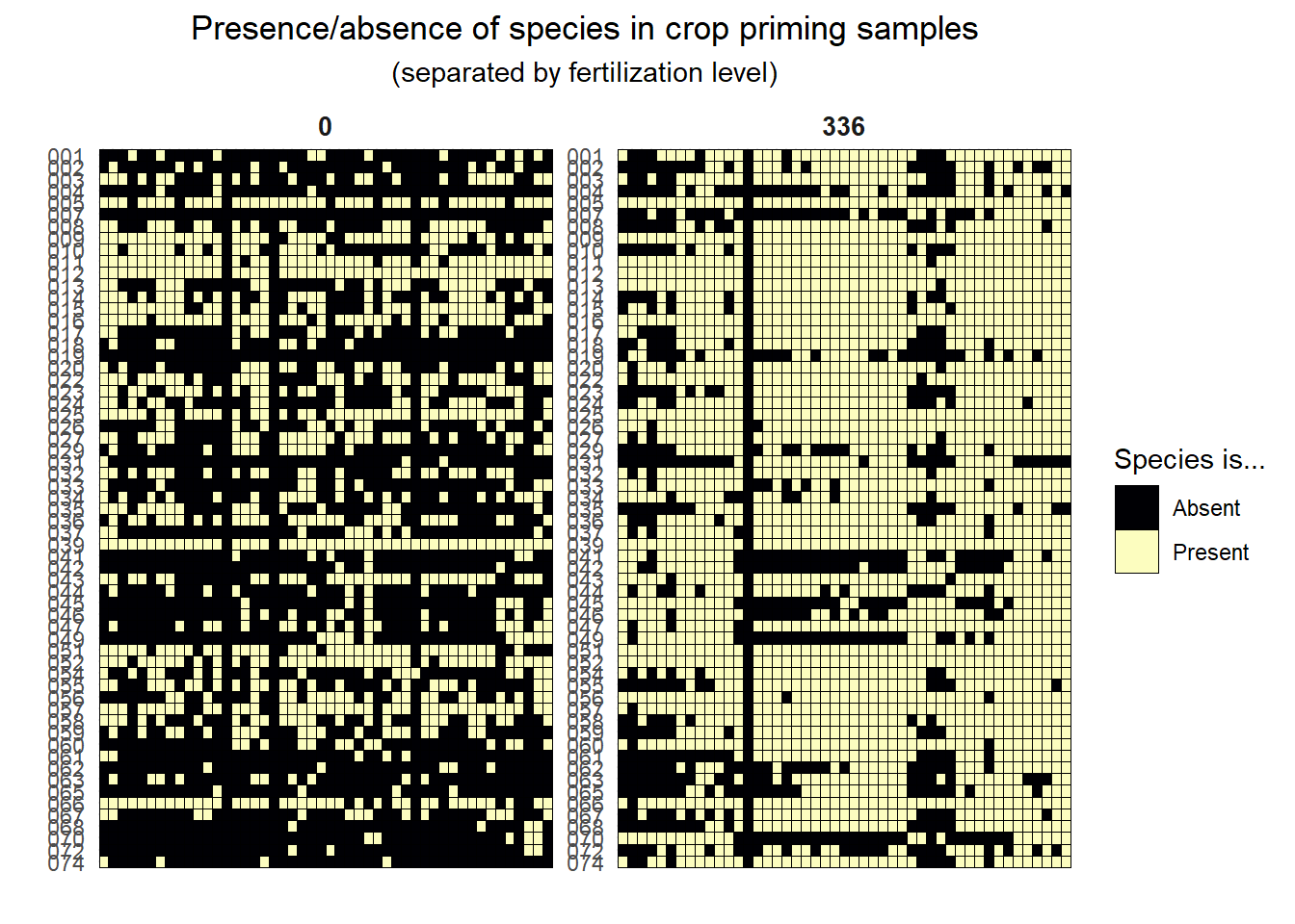
We can plot this data to get an idea of the richness in the samples. We’ll also separate the data by fertilization level to get an idea of the relationship between that treatment and presence/absence.
amoA_presence_absence %>%rownames_to_column(var ="sample_id") %>%pivot_longer(cols = amoA.001:amoA.074, names_to ="amoA", values_to ="presence") %>%mutate(amoA =str_sub(amoA, -3),presence =as.factor(presence)) %>%left_join(metadata %>%rownames_to_column(var ="sample_id")) %>%ggplot(aes(sample_id, amoA, fill = presence)) +geom_tile(color ="black") +labs(x ="",y ="",fill ="Species is...",title ="Presence/absence of species in crop priming samples",subtitle ="(separated by fertilization level)" ) +# scale_fill_manual(values = pa_cols)scale_fill_viridis_d(labels =c("Absent", "Present"),begin =0, end =1,option ="magma") +theme(axis.text.x =element_blank(),plot.title =element_text(hjust =0.5),plot.subtitle =element_text(hjust =0.5),# strip.background = element_rect(color = "black", fill = "NA", size = 1),strip.text =element_text(size =10, face ="bold") ) +scale_y_discrete(limits = rev) +facet_wrap(~ fert_level, scales ="free")